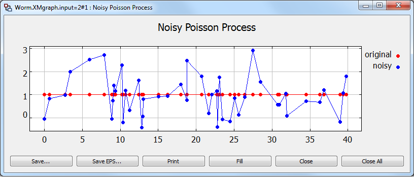
Now you can execute the simulation but bear in mind that both PTcl and parameter file have to be at the same location. The figures below show the model representation within the MLDesigner GUI and the result of the simulation.
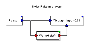
Worm system
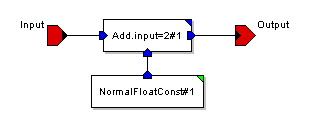
WormGuts module